Variant set plot
This tutorial shows how to compare effect sizes for a fixed set of variants across multiple GWAS studies using gl.SumstatsSet and plot_effect(). For the full parameter reference, see Variant Set Plot.
In development
SumstatsSet and plot_effect() are under active development. The development notebook lives at examples/_development/variant_set/visualization_variant_set.ipynb.
Basic variant set plot
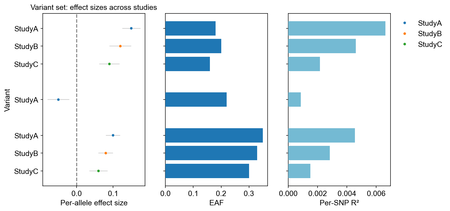
Load two or more Sumstats objects, pass a list of variant IDs to SumstatsSet, then call plot_effect() to draw a forest-style panel grouped by variant.
Example
rows_a = [
    {"CHR": 1, "POS": 100, "EA": "A", "NEA": "G", "BETA": 0.10, "SE": 0.02, "P": 1e-6, "EAF": 0.35, "SNPID": "1:100:A:G"},
    {"CHR": 2, "POS": 200, "EA": "C", "NEA": "T", "BETA": -0.05, "SE": 0.03, "P": 1e-4, "EAF": 0.22, "SNPID": "2:200:C:T"},
    {"CHR": 7, "POS": 500000, "EA": "G", "NEA": "A", "BETA": 0.15, "SE": 0.025, "P": 1e-8, "EAF": 0.18, "SNPID": "rs7890"},
]
rows_b = [
    {"CHR": 1, "POS": 100, "EA": "A", "NEA": "G", "BETA": 0.08, "SE": 0.02, "P": 5e-8, "EAF": 0.33, "SNPID": "1:100:A:G"},
    {"CHR": 7, "POS": 500000, "EA": "G", "NEA": "A", "BETA": 0.12, "SE": 0.03, "P": 1e-6, "EAF": 0.20, "SNPID": "rs7890"},
]
rows_c = [
    {"CHR": 1, "POS": 100, "EA": "A", "NEA": "G", "BETA": 0.06, "SE": 0.025, "P": 1e-4, "EAF": 0.30, "SNPID": "1:100:A:G"},
    {"CHR": 7, "POS": 500000, "EA": "G", "NEA": "A", "BETA": 0.09, "SE": 0.028, "P": 1e-5, "EAF": 0.16, "SNPID": "rs7890"},
]

def make_sumstats(rows):
    return gl.Sumstats(
        sumstats=pd.DataFrame(rows),
        chrom="CHR", pos="POS", ea="EA", nea="NEA",
        snpid="SNPID", beta="BETA", se="SE", p="P", eaf="EAF",
        verbose=False,
    )

studies = {"StudyA": make_sumstats(rows_a), "StudyB": make_sumstats(rows_b), "StudyC": make_sumstats(rows_c)}
variant_set = [[1, 100], "2:200:C:T", "rs7890"]

sset = gl.SumstatsSet(studies, variant_set=variant_set, verbose=False)
sset.data[["STUDY", "SNPID", "BETA", "SE", "EAF"]]
Example
Variant ID formats
variant_set accepts several identifier styles. Matching uses SNPID for strings and CHR + POS for coordinate pairs.
| Format | Example | Matches by |
|---|---|---|
| rsID | "rs7890" |
Exact SNPID |
| CHR + POS | [1, 100] |
CHR and POS |
| Variant ID string | "1:100:A:G" |
Parsed CHR and POS |
Example
Load studies from a glob pattern
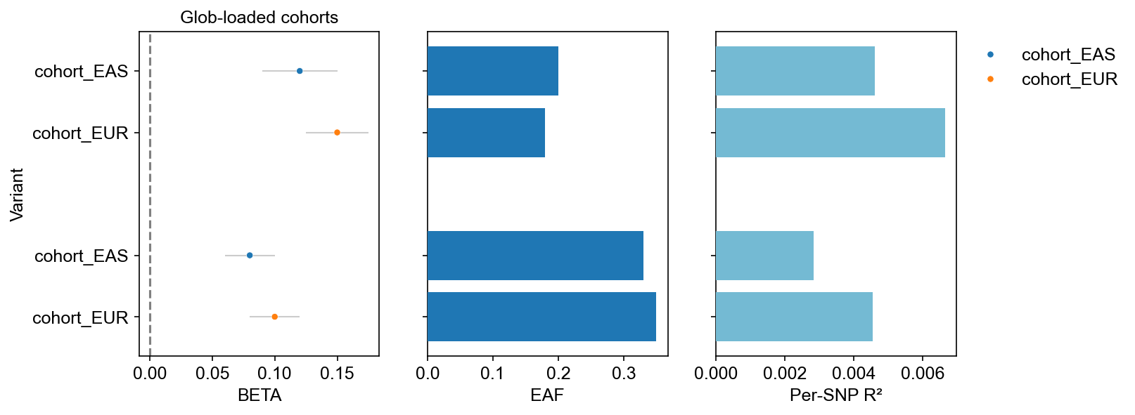
When many cohort files share the same column layout, pass a glob pattern instead of a dictionary. Study names are derived from filenames (e.g. cohort_EUR.txt → cohort_EUR).
Example
Side panels: EAF and SNPR2
When EAF or SNPR2 columns are present, plot_effect() adds optional horizontal bar panels beside the main effect panel. Panels are skipped automatically if the column is missing.
| Panel | Column | Description |
|---|---|---|
| EAF | EAF |
Effect-allele frequency |
| SNPR2 | SNPR2 |
Per-variant R² (see Per-SNP R2 and F) |
Disable a panel with eaf_panel=False or snpvar_panel=False.
Related plots
| Function | Use case |
|---|---|
compare_effect() |
Scatter comparing two studies (auto lead extraction) |
plot_forest() |
Meta-analysis forest plot with combined estimate |
plot_lead_overlap() |
Venn/UpSet of lead locus overlap across studies |